Decomposition Module (API Reference)
The scikitplot.decomposition module includes plots built specifically
for scikit-learn estimators that are used for dimensionality reduction
e.g. PCA. You can use your own estimators, but these plots assume specific
properties shared by scikit-learn estimators. The specific requirements are
documented per function.
-
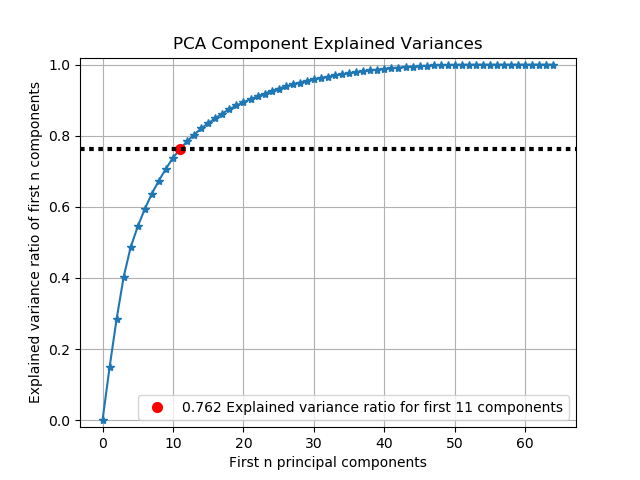
scikitplot.decomposition.plot_pca_component_variance(clf, title=u'PCA Component Explained Variances', target_explained_variance=0.75, ax=None, figsize=None, title_fontsize=u'large', text_fontsize=u'medium')¶ Plots PCA components’ explained variance ratios. (new in v0.2.2)
Parameters: - clf – PCA instance that has the
explained_variance_ratio_attribute. - title (string, optional) – Title of the generated plot. Defaults to “PCA Component Explained Variances”
- target_explained_variance (float, optional) – Looks for the minimum number of principal components that satisfies this value and emphasizes it on the plot. Defaults to 0.75
- ax (
matplotlib.axes.Axes, optional) – The axes upon which to plot the curve. If None, the plot is drawn on a new set of axes. - figsize (2-tuple, optional) – Tuple denoting figure size of the plot
e.g. (6, 6). Defaults to
None. - title_fontsize (string or int, optional) – Matplotlib-style fontsizes. Use e.g. “small”, “medium”, “large” or integer-values. Defaults to “large”.
- text_fontsize (string or int, optional) – Matplotlib-style fontsizes. Use e.g. “small”, “medium”, “large” or integer-values. Defaults to “medium”.
Returns: - The axes on which the plot was
drawn.
Return type: ax (
matplotlib.axes.Axes)Example
>>> import scikitplot as skplt
>>> pca = PCA(random_state=1)
>>> pca.fit(X)
>>> skplt.decomposition.plot_pca_component_variance(pca)
<matplotlib.axes._subplots.AxesSubplot object at 0x7fe967d64490>
>>> plt.show()
- clf – PCA instance that has the
-
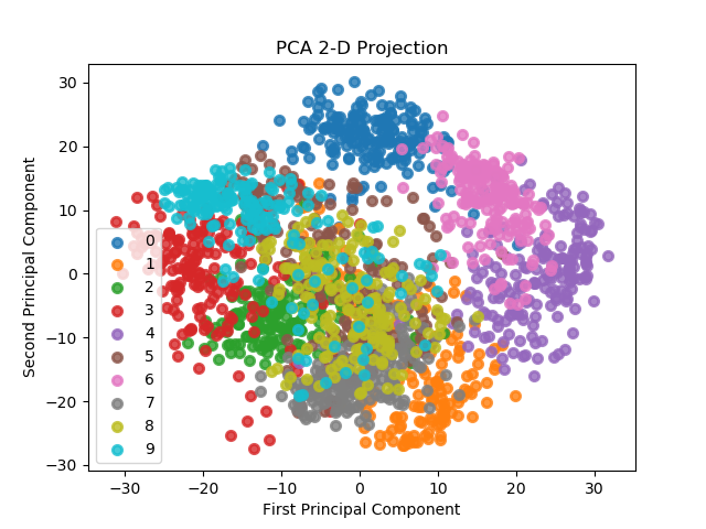
scikitplot.decomposition.plot_pca_2d_projection(clf, X, y, title=u'PCA 2-D Projection', ax=None, figsize=None, cmap=u'Spectral', title_fontsize=u'large', text_fontsize=u'medium')¶ Plots the 2-dimensional projection of PCA on a given dataset.
Parameters: - clf – Fitted PCA instance that can
transformgiven data set into 2 dimensions. - X (array-like, shape (n_samples, n_features)) – Feature set to project, where n_samples is the number of samples and n_features is the number of features.
- y (array-like, shape (n_samples) or (n_samples, n_features)) – Target relative to X for labeling.
- title (string, optional) – Title of the generated plot. Defaults to “PCA 2-D Projection”
- ax (
matplotlib.axes.Axes, optional) – The axes upon which to plot the curve. If None, the plot is drawn on a new set of axes. - figsize (2-tuple, optional) – Tuple denoting figure size of the plot
e.g. (6, 6). Defaults to
None. - cmap (string or
matplotlib.colors.Colormapinstance, optional) – Colormap used for plotting the projection. View Matplotlib Colormap documentation for available options. https://matplotlib.org/users/colormaps.html - title_fontsize (string or int, optional) – Matplotlib-style fontsizes. Use e.g. “small”, “medium”, “large” or integer-values. Defaults to “large”.
- text_fontsize (string or int, optional) – Matplotlib-style fontsizes. Use e.g. “small”, “medium”, “large” or integer-values. Defaults to “medium”.
Returns: - The axes on which the plot was
drawn.
Return type: ax (
matplotlib.axes.Axes)Example
>>> import scikitplot as skplt
>>> pca = PCA(random_state=1)
>>> pca.fit(X)
>>> skplt.decomposition.plot_pca_2d_projection(pca, X, y)
<matplotlib.axes._subplots.AxesSubplot object at 0x7fe967d64490>
>>> plt.show()
- clf – Fitted PCA instance that can